4 Isotopic niche overlaps

4.1 Libraries

library(nicheROVER)
library(ggplot2)
library(dplyr)

4.2 Data

data <- read.csv("data/glm.csv", header = T)
colnames(data)[6:7] <- c("iso1", "iso2")
global <- subset(data, select = c(sp, iso1, iso2))
global$group <- factor(global$sp, labels = c(1:3))
global$community <- 1
head(global)

4.3 Projections of niche regions

Basic parameters for plotting:

global_colors <- c('#1f77b4', '#ff7f0e', '#2ca02c')
xlims <- c(min(global$iso2)-0.5, max(global$iso2)+0.5)
ylims <- c(min(global$iso1)-0.5, max(global$iso1)+0.5)
species <- unique(global$sp)

nicheROVER performs a Bayesian estimation of the isotopic niche and then calculates the probability of its overlap with the isotopic niche of another; i.e., how probable is to find an individual of one species in the isotopic space of another. Thus, this overlap is directional and more informative than the traditional, non-directional, geometric approximation (Swanson et al. 2015).

# Number of posterior samples
nsamples <- 1000

# Estimates of the isotopic niche
bpar <- tapply(1:nrow(global), global$sp,
               function(ii) niw.post(nsamples = nsamples,
                                     X = global[ii, 2:3]))

bdata <- tapply(1:nrow(global),
                global$sp,
                function(ii) X = global[ii, 2:3])

Plot of the isotopic niches:

niche.plot(niche.par = bpar,
           niche.data = bdata,
           pfrac = 0.05,
           iso.names = expression(delta^{15}*N, delta^{13}*C),
           col = global_colors,
           xlab = expression ("Isotope ratio (‰)"))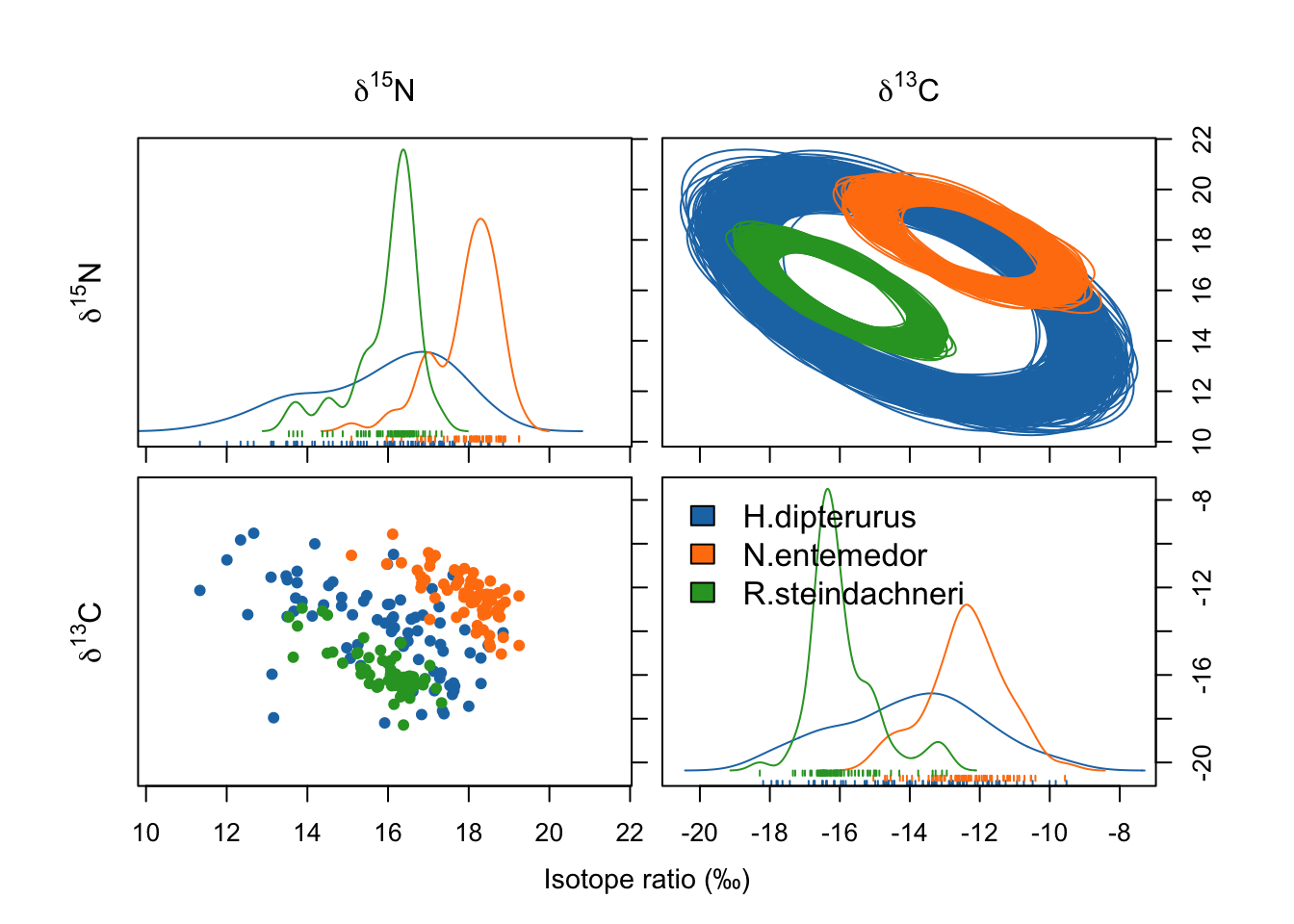

Mean overlaps with the means for 95% and 99% ellipses:

over.stat <- overlap(bpar,
                     nreps = nsamples,
                     nprob = 1e3,
                     alpha = c(0.95, 0.99))
over.mean <- apply(over.stat,
                   c(1:2, 4),
                   mean)*100
round(over.mean)

, , alpha = 95%

                 Species B
Species A         H.dipterurus N.entemedor R.steindachneri
  H.dipterurus              NA           9              25
  N.entemedor               71          NA               0
  R.steindachneri          100           0              NA

, , alpha = 99%

                 Species B
Species A         H.dipterurus N.entemedor R.steindachneri
  H.dipterurus              NA          14              35
  N.entemedor               96          NA               0
  R.steindachneri          100           0              NA

95% Highest density intervals for the overlaps

over.cred <- apply(over.stat*100,
                   c(1:2, 4),
                   quantile,
                   prob = c(.025, .975),
                   na.rm = TRUE)
round(over.cred[,,,1]) # display alpha = .95 niche region

, , Species B = H.dipterurus

       Species A
        H.dipterurus N.entemedor R.steindachneri
  2.5%            NA          41              98
  97.5%           NA          96             100

, , Species B = N.entemedor

       Species A
        H.dipterurus N.entemedor R.steindachneri
  2.5%             4          NA               0
  97.5%           15          NA               0

, , Species B = R.steindachneri

       Species A
        H.dipterurus N.entemedor R.steindachneri
  2.5%            17           0              NA
  97.5%           33           0              NA

Plot with the posterior distributions of the niche overlaps:

over.stat <- overlap(bpar, nreps = nsamples, nprob = 1e3, alpha = .95)
#cairo_pdf("nicheROVER.pdf", width = 7, height = 7/1.61, family = "Times")
overlap.plot(over.stat, col = global_colors,
             mean.cred.col = "firebrick",
             equal.axis = TRUE,
             xlab = "Overlap Probability (%)")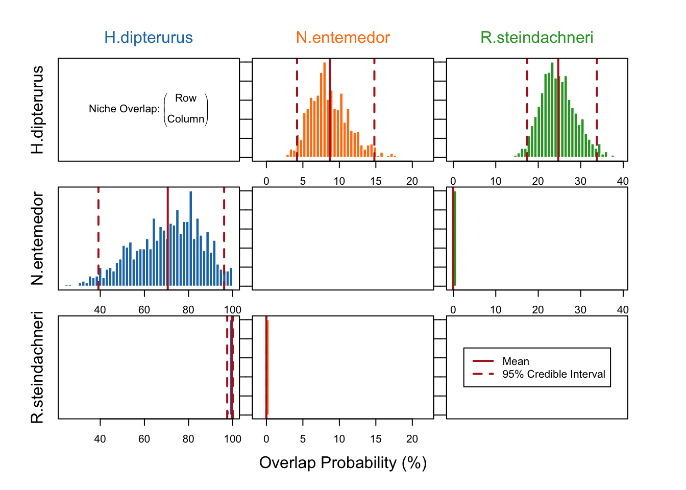

#dev.off()