3  Amplitudes and comparisons of the isotopic niches

3.1 Libraries

library(SIBER)
library(ggplot2)
library(ggExtra)
library(ggConvexHull)
library(HDInterval)
library(mcmcplots)
library(ggmcmc)
library(coda)
library(lattice)
library(MCMCvis)
library(bayesplot)

3.2 Data loading

data <- read.table("data/glm.csv", sep = ",", header = T)
colnames(data)[6:7] <- c("iso1", "iso2")

3.3 “Global” SIBER:

3.3.1 Dataset arrangement

global <- subset(data, select = c(sp, iso1, iso2))
global$group <- factor(global$sp, labels = c(1:3))
global$community <- 1
global

3.3.2 Basic plot

Parameters and basic information

global_colors <- c('#1f77b4', '#ff7f0e', '#2ca02c')
xlims <- c(min(global$iso2)-0.5, max(global$iso2)+0.5)
ylims <- c(min(global$iso1)-0.5, max(global$iso1)+0.5)
species <- unique(global$sp)

Plot

glob_ellipses <- ggplot(data = global, aes(x = iso2, y = iso1, color = as.factor(group))) +
                 geom_point(alpha = 0.7) +
                 stat_ellipse(level = 0.4) +
                 geom_convexhull(fill = NA, linetype = "dashed", alpha = 0.05) +
                 scale_color_manual(values = global_colors, name = "Species", labels = species) +
                 scale_x_continuous(limits = xlims, breaks = c(seq(-18, -8, 2))) +
                 scale_y_continuous(limits = ylims, breaks = c(seq(10, 20, 2))) +
                 labs(title = element_blank(),
                      x = expression({delta}^13*C~'(\u2030)'),
                      y = expression({delta}^15*N~'(\u2030)')) +
                 theme_bw() +
                 theme(aspect.ratio = 1,
                       panel.grid.major = element_blank(),
                       panel.grid.minor = element_blank(),
                       legend.position = c(0.20, 0.17),
                       legend.background = element_blank())

# cairo_pdf("output/SIBER/global/global_ellipses.pdf",
#           family = "Times", height = 3.5, width = 3.5)
glob_ellipses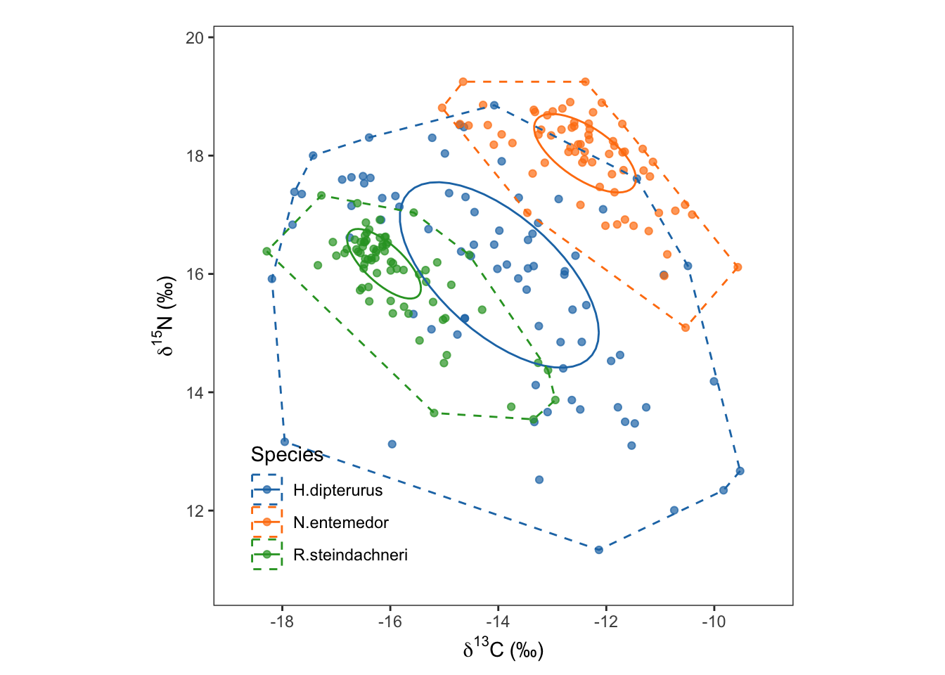

# dev.off()

3.3.3 Fitting the Bayesian Bi-variate Normal models:

Creation of the SIBER object:

siber_glob <- createSiberObject(global[,2:5])

Parameters of the MCMC:

parms <- list()
parms$n.iter   <- 20000    
parms$n.burnin <- 25000   
parms$n.thin   <- 1          
parms$n.chains <- 3
parms$save.output <- TRUE
parms$save.dir <- paste(getwd(),"/output/SIBER/global", sep = "")

Prior distributions:

priors <- list()
priors$R <- 1 * diag(2)
priors$k <- 2
priors$tau.mu <- 1.0E-3

Sampling of the posterior distributions:

ellipses.posterior <- siberMVN(siber_glob, parms, priors)

Compiling model graph
   Resolving undeclared variables
   Allocating nodes
Graph information:
   Observed stochastic nodes: 81
   Unobserved stochastic nodes: 3
   Total graph size: 96

Initializing model

Compiling model graph
   Resolving undeclared variables
   Allocating nodes
Graph information:
   Observed stochastic nodes: 69
   Unobserved stochastic nodes: 3
   Total graph size: 84

Initializing model

Compiling model graph
   Resolving undeclared variables
   Allocating nodes
Graph information:
   Observed stochastic nodes: 74
   Unobserved stochastic nodes: 3
   Total graph size: 89

Initializing model

3.3.3.1 Diagnostics:

Cycling through every model to extract information:

all_files <- dir(parms$save.dir, full.names = T)
model_files <- all_files[grep("jags_output", all_files)]

model_summary <- list()

for (i in seq_along(model_files)) {
  load(model_files[i])
  
  mcmc_list <- coda::as.mcmc(do.call("cbind", output))
  
  model_summary[[i]] <- MCMCsummary(output,
                                    params = "all",
                                    probs = c(0.025, 0.975),
                                    round = 3)
  MCMCtrace(output,
            params = "all",
            iter = parms$n.iter,
            Rhat = T,
            n.eff = T,
            ind = T,
            type = "density",
            open_pdf = F,
            filename = sprintf("output/SIBER/global/MCMCtrace_%d", i))
}

Autocorrelation plots:

# cairo_pdf("output/SIBER/global_autocorr.pdf",
#           family = "Times", height = 10, width = 12)
gridExtra::grid.arrange(mcmc_acf(ellipses.posterior[1]) + labs(title = species[1]),
                        mcmc_acf(ellipses.posterior[2]) + labs(title = species[2]),
                        mcmc_acf(ellipses.posterior[3]) + labs(title = species[3]),
                        nrow = 3)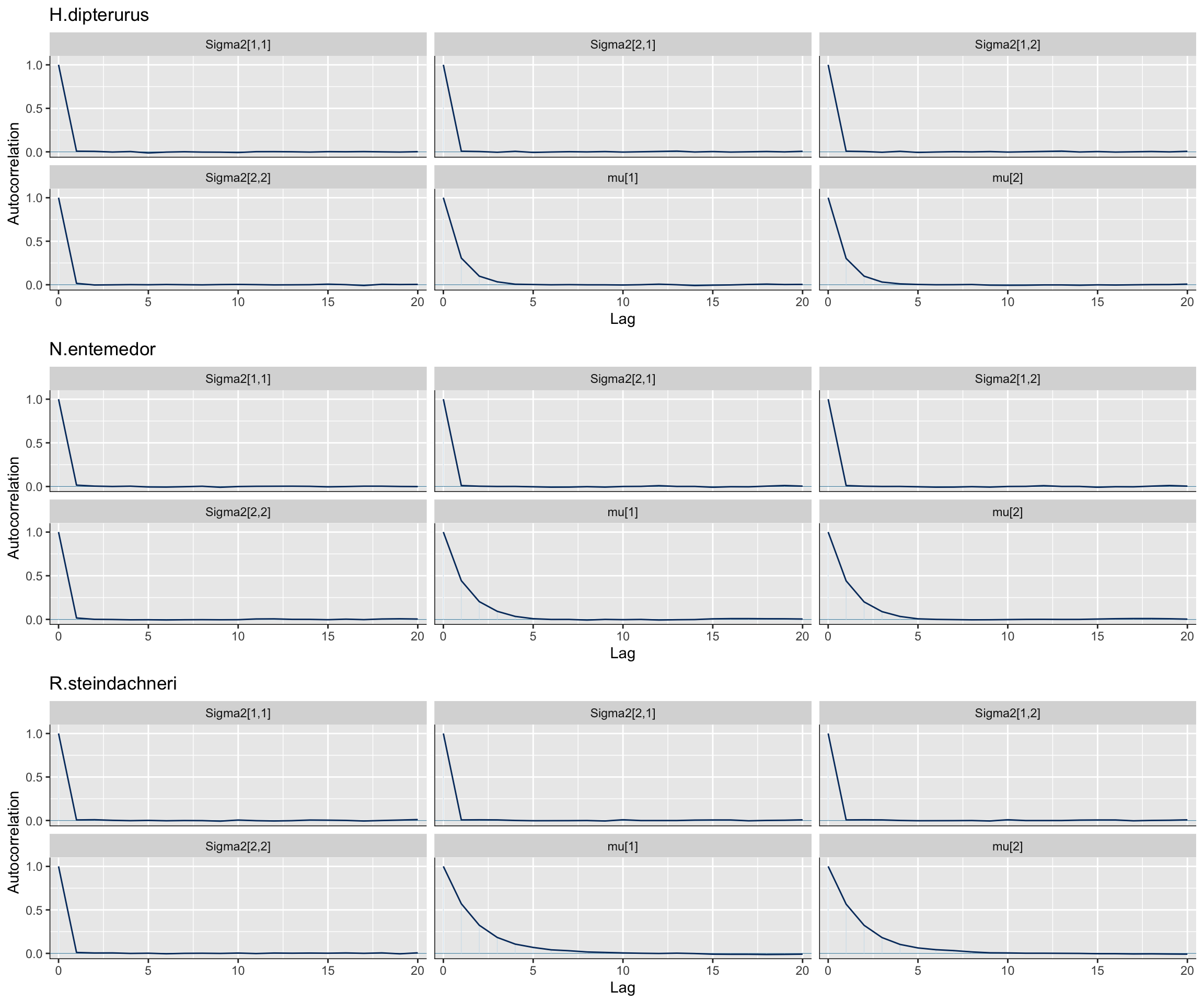

#dev.off()

Summaries. Gelman-Rubick Statistics (Rhat) exactly equal to 1 and effective sample sizes > 2000 for every parameter:

for (i in seq_along(model_files)) {
  load(model_files[i])
  print(species[i])
  print(model_summary[[i]])
}

[1] "H.dipterurus"
              mean    sd   2.5%  97.5% Rhat n.eff
Sigma2[1,1]  1.025 0.165  0.751  1.393    1 60000
Sigma2[2,1] -0.557 0.132 -0.851 -0.331    1 59779
Sigma2[1,2] -0.557 0.132 -0.851 -0.331    1 59779
Sigma2[2,2]  1.025 0.165  0.753  1.392    1 58288
mu[1]        0.000 0.112 -0.221  0.220    1 31856
mu[2]        0.000 0.112 -0.220  0.221    1 31680
[1] "N.entemedor"
              mean    sd   2.5%  97.5% Rhat n.eff
Sigma2[1,1]  1.030 0.180  0.734  1.434    1 58420
Sigma2[2,1] -0.684 0.152 -1.025 -0.432    1 58657
Sigma2[1,2] -0.684 0.152 -1.025 -0.432    1 58657
Sigma2[2,2]  1.030 0.180  0.736  1.440    1 58409
mu[1]        0.001 0.121 -0.240  0.239    1 23172
mu[2]       -0.001 0.122 -0.240  0.238    1 23062
[1] "R.steindachneri"
              mean    sd   2.5%  97.5% Rhat n.eff
Sigma2[1,1]  1.028 0.174  0.743  1.420    1 59100
Sigma2[2,1] -0.773 0.154 -1.119 -0.519    1 58438
Sigma2[1,2] -0.773 0.154 -1.119 -0.519    1 58438
Sigma2[2,2]  1.029 0.174  0.742  1.426    1 57750
mu[1]       -0.002 0.118 -0.234  0.229    1 16294
mu[2]        0.002 0.118 -0.228  0.234    1 16515

3.3.3.2 Inferences

Generation of the ellipses:

sea_b <- siberEllipses(ellipses.posterior)
summary(sea_b)

       V1               V2              V3       
 Min.   : 6.193   Min.   :1.323   Min.   :1.077  
 1st Qu.: 8.875   1st Qu.:1.971   1st Qu.:1.541  
 Median : 9.555   Median :2.136   Median :1.666  
 Mean   : 9.636   Mean   :2.156   Mean   :1.681  
 3rd Qu.:10.311   3rd Qu.:2.318   3rd Qu.:1.804  
 Max.   :15.689   Max.   :3.721   Max.   :3.167  

Graphical comparisons. First, transform the object to a data.frame and melt it to long format:

sea_bt <- reshape2::melt(as.data.frame(sea_b))

No id variables; using all as measure variables

colnames(sea_bt) <- c("sp", "SEAb")
head(sea_bt)

Get the HDI for each species:

hdi <- as.data.frame(t(apply(sea_b, 2, FUN = HDInterval::hdi)))
hdi <- cbind(hdi, means = t(as.data.frame(t(apply(sea_b, 2, FUN = mean)))))
hdi["sp"] <- row.names(hdi)
hdi

Violin plot with the posterior distributions of the SEAb:

seab_global <- ggplot() +
               geom_violin(data = sea_bt, aes(x = sp, y = SEAb, fill = sp, color = sp),
                           show.legend = F, alpha = 0.3) +
               geom_boxplot(data = sea_bt,
                            aes(x = sp, y = SEAb, fill = sp, color = sp),
                            alpha = 0.5, width = 0.05, notch = T, show.legend = F,
                            outlier.shape = NA, coef = 0) +
               scale_fill_manual(values = global_colors) +
               scale_color_manual(values = global_colors) +
               geom_linerange(data = hdi,
                              aes(x = sp, ymin = lower, ymax = upper, color = sp),
                              show.legend = F) +
               theme_bw()+
               theme(aspect.ratio = 1,
                     panel.grid.major = element_blank(),
                     panel.grid.minor = element_blank(),
                     legend.position = c(0.2, 0.15),
                     legend.background = element_blank()) +
               labs(x = "Species",
                    y = expression("SEAb " ('\u2030' ^2) )) +
               scale_x_discrete(labels = species)
# cairo_pdf("output/SIBER/global/global_seab.pdf",
#           family = "Times", height = 3.5, width = 3.5)
seab_global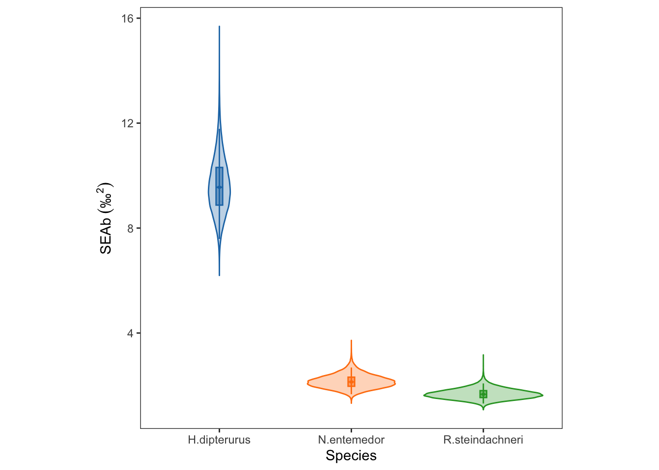

#dev.off()

Posterior Differences:

# Define the comparisons
comps <- expand.grid(a = unique(as.integer(global$group)),
                     b = unique(as.integer(global$group)))
comps <- comps[(comps$a != comps$b & comps$b > comps$a), ]
comps <- comps[order(comps$a),]

# Put the results in different objects:
diffs <- data.frame()
diff_glob <- data.frame()
p_sup <- data.frame()
for (i in seq_along(comps$a)) {
  a <- comps$a[i]
  b <- comps$b[i]
  comp <- paste(species[a], "-", species[b])
  diff <- sea_b[, a] - sea_b[, b]
  sup <- subset(diff, diff>0, select = diff)
  
  diffs <- rbind(diffs,
                 data.frame(comp = comp,
                            diff = diff))
  diff_glob <- rbind(diff_glob,
                     data.frame(comp = comp,
                                mean = mean(diff),
                                IQr = t(HDInterval::hdi(diff, credMass = 0.5)),
                                hdi = t(HDInterval::hdi(diff, credMass = 0.95))
                                )
                     )
  p_sup <- rbind(p_sup,
                 data.frame(comp = comp,
                            p_sup = (length(sup)/length(diff))*100))
}

diff_glob$comp <- factor(diff_glob$comp, ordered = T)

HDIs of differences

diff_glob["keys"] <- factor(c("HD-NE", "HD-RS", "NE-RS"), ordered = T)
diff_glob

Probabilities of differences:

p_sup

Forestplot of the \(HDI_{95\%}\) of the differences

global_forest <- ggplot(data = diff_glob) +
                 geom_vline(xintercept = 0, linetype = "dashed", color = "#C9C8C8", size = 1.2) +
                 geom_linerange(aes(y = factor(comp, ordered = T),
                                    xmin = IQr.lower, xmax = IQr.upper),
                                color = global_colors[1], size = 1) +
                 geom_linerange(aes(y = factor(comp, ordered = T),
                                    xmin = hdi.lower, xmax = hdi.upper),
                                color = global_colors[1]) +
                 geom_point(aes(x = mean, y = factor(comp, ordered = T)),
                            color = global_colors[1],
                            fill = "white", size = 1.5, shape = 21) +
                 theme_bw() +
                 theme(aspect.ratio = 1,
                       panel.grid.major = element_blank(),
                       panel.grid.minor = element_blank(),
                       legend.position = c(0.2, 0.15),
                       legend.background = element_blank()) +
                 labs(title = expression("Differences in SEAB " ('\u2030' ^2)),
                      x = element_blank(),
                      y = element_blank())

# cairo_pdf("output/SIBER/global/global_forest.pdf",
#           family = "Times", height = 4, width = 4)
global_forest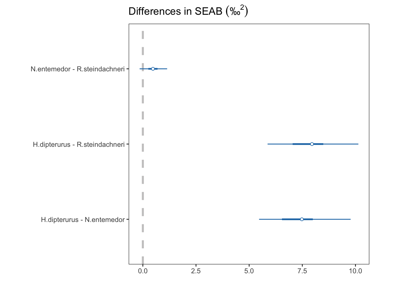

# dev.off()

3.3.3.3 Eccentricity and theta

Eccentricities represent the elongation of the ellipse, that is, how far they are from a perfect circle (0 eccentricity). Lower values indicate a rounder ellipse, while higher values indicate a more elongated ellipse.

mat_ecc <- function(x) {
  mat <- matrix(x, 2, 2)
  ecc <- sigmaSEA(mat)$ecc
  return(ecc)
}

mat_theta <- function(x){
  mat <- matrix(x, 2, 2)
  theta <- sigmaSEA(mat)$theta
  return(theta)
}

ecc <- data.frame()
for (sp in seq_along(ellipses.posterior)) {
  ecc <- rbind(ecc,
               data.frame(sp = species[sp],
                          ecc = apply(ellipses.posterior[[sp]][,1:4], 1, mat_ecc),
                          theta = apply(ellipses.posterior[[sp]][,1:4], 1, mat_theta)))
}

ec <- ecc %>% group_by(sp) %>% summarise(IQR.lower = hdi(ecc, credMass = 0.5)[1],
                                         IQR.upper = hdi(ecc, credMass = 0.5)[2],
                                         hdi.lower = hdi(ecc)[1],
                                         hdi.upper = hdi(ecc)[2],
                                         mean = mean(ecc))
ec

ggplot(data = ecc, aes(x = sp, y = ecc, group = sp, color = factor(sp))) +
  geom_violin(fill = NA, show.legend = F) +
  geom_point(aes(x = sp, y = mean), data = ec, show.legend = F) +
  #geom_errorbar(aes(x = sp, ymin = IQ.lower, ymax = IQ.upper, group = sp), data = ag) +
  geom_boxplot(width = 0.1, show.legend = F) +
  theme_bw() +
  labs(title = "SEAB Eccentricity",
       x = element_blank(),
       y = element_blank()) +
  scale_color_manual(values = global_colors) +
  theme(aspect.ratio = 1,
                       panel.grid.major = element_blank(),
                       panel.grid.minor = element_blank(),
                       legend.position = c(0.15, 0.1),
                       legend.background = element_blank())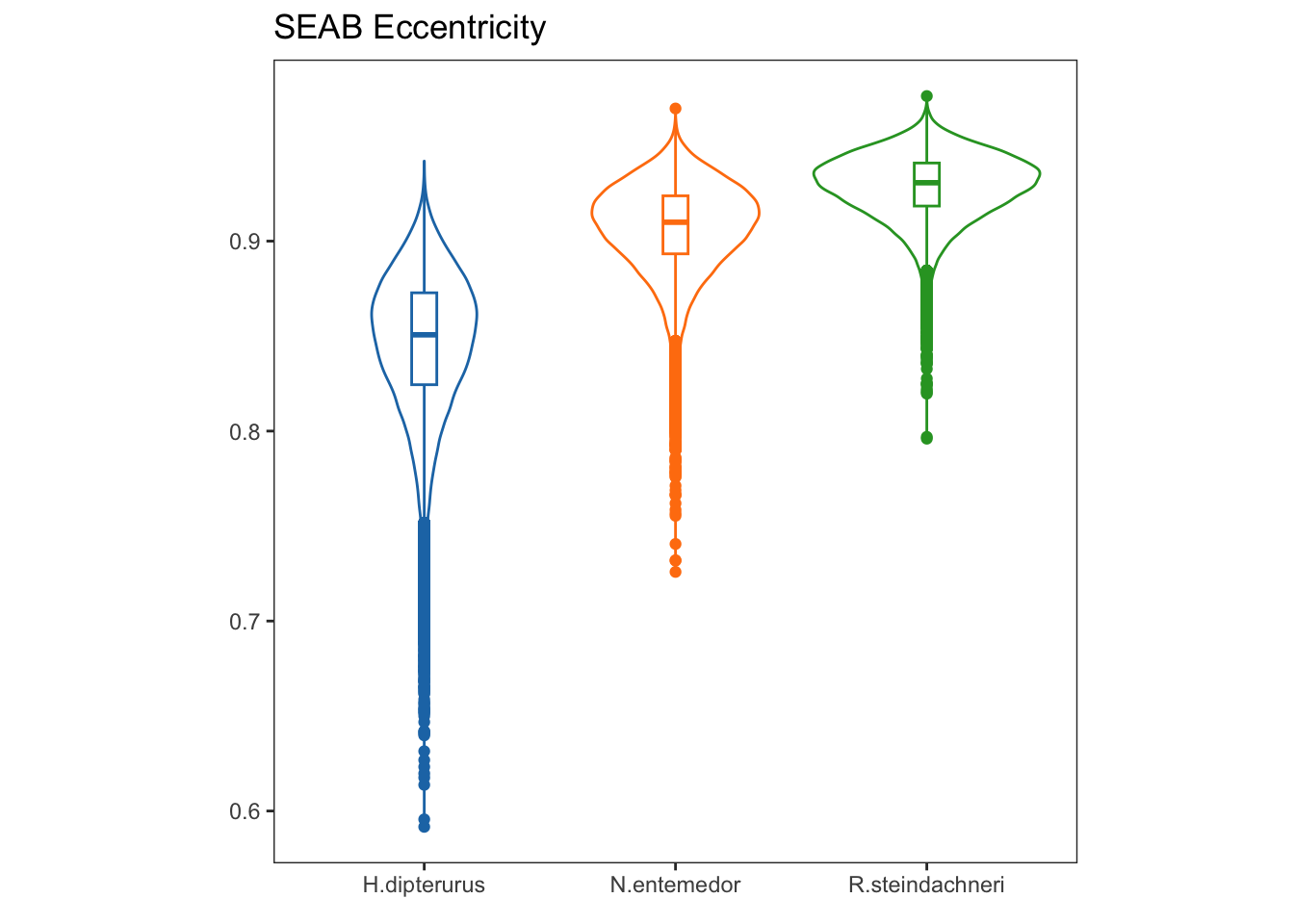

Theta, on the other hand, is the angle of the semi-major axis of the SEA and the x axis; i.e., the angle of the deformation. Values close to 0 show a higher dispersion in \(\delta^{13}C\), while values close to 90 show a higher dispersion in \(\delta^{15}N\):

th <- ecc %>% group_by(sp) %>% summarise(IQR.lower = hdi(theta, credMass = 0.5)[1],
                                         IQR.upper = hdi(theta, credMass = 0.5)[2],
                                         hdi.lower = hdi(theta)[1],
                                         hdi.upper = hdi(theta)[2],
                                         mean = mean(theta))
th

ggplot(data = ecc, aes(x = sp, y = theta, group = sp, color = factor(sp))) +
  geom_violin(fill = NA, show.legend = F) +
  geom_point(aes(x = sp, y = mean), data = ec, show.legend = F) +
  #geom_errorbar(aes(x = sp, ymin = IQ.lower, ymax = IQ.upper, group = sp), data = ag) +
  geom_boxplot(width = 0.1, show.legend = F) +
  theme_bw() +
  labs(title = "SEAB theta",
       x = element_blank(),
       y = element_blank()) +
  scale_color_manual(values = global_colors) +
  theme(aspect.ratio = 1,
                       panel.grid.major = element_blank(),
                       panel.grid.minor = element_blank(),
                       legend.position = c(0.15, 0.1),
                       legend.background = element_blank())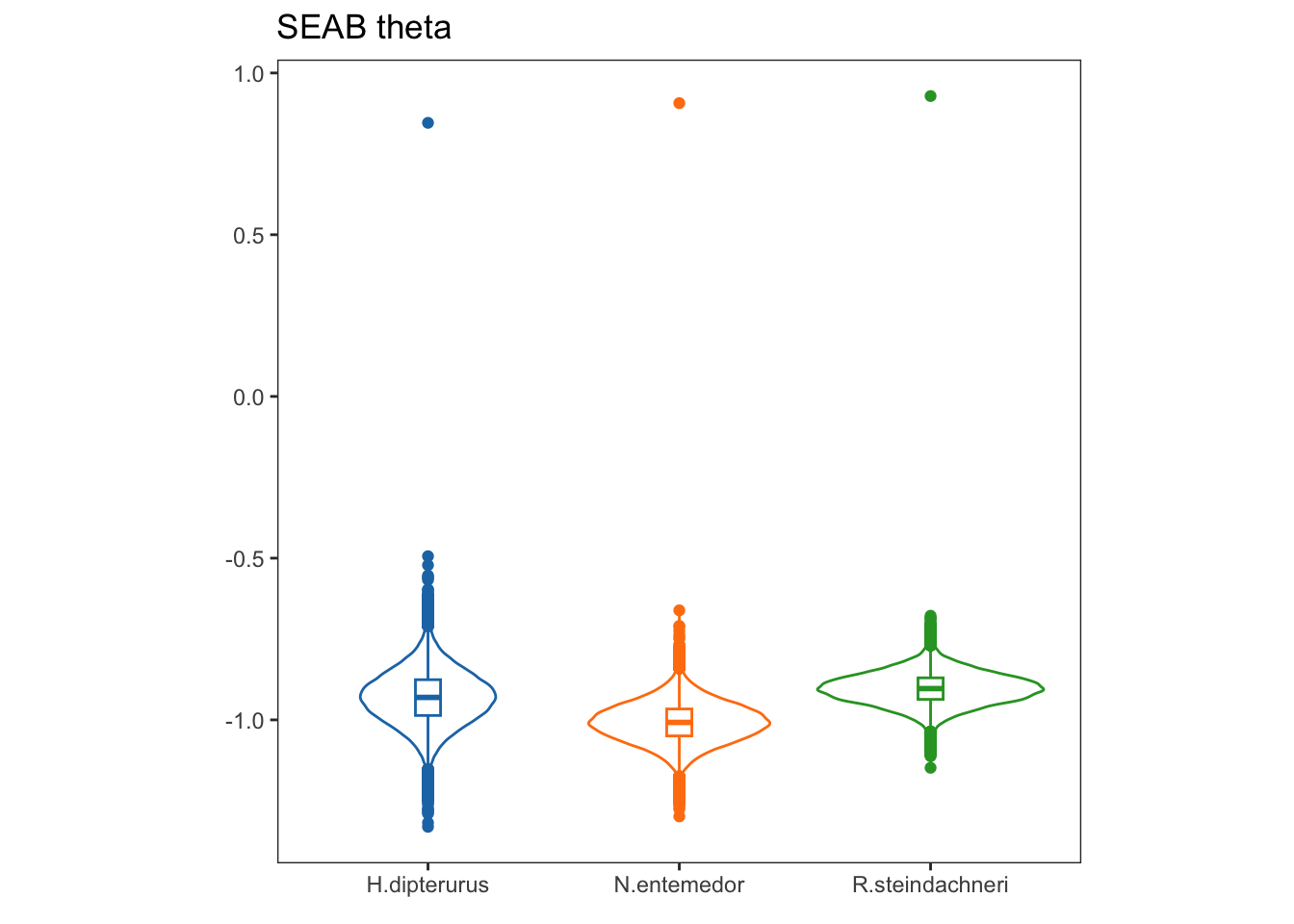

3.4 Intra-specific analyses

Basic dataset to extract every case:

full_set <- subset(data,
                   select = c(sp, temporada, sexo, estadio, iso1, iso2))

colnames(full_set) <- c("Species", "Season", "Sex", "Maturity", "iso1", "iso2")

head(full_set)

3.4.1 Custom wrapper around SIBER:

custom_siber <- function(data, var_col, lbls, sp_col, colors, gp_label,
                         n.burnin = 30000, n.iter = 2000){
  
  subdata <- data[,c(sp_col, var_col, "iso1", "iso2")]
  subdata$group <- factor(subdata[,var_col], labels = seq_along(lbls))
  subdata$community <- 1
  
  species <- unique(data[, sp_col])
  
  # Global directory for the variable
  wd <- paste(getwd(), "/output/SIBER/", var_col, sep = "")
  
  # If the directory does not exist, create it:
  if (dir.exists(wd) == F) {dir.create(wd)}
  
  # Empty lists to store the results:
  siber_objs <- list()
  ellipses <- list()

  summaries <- list()
  autocorr_plots <- list()
  
  sea_b <- list()
  sea_bt <- data.frame()
  hdis <- data.frame()
  ecc <- data.frame()
  
  # Posterior differences
  # Define the comparisons
  comps <- expand.grid(a = unique(as.integer(subdata$group)),
                       b = unique(as.integer(subdata$group)))
  
  comps <- comps[(comps$a != comps$b & comps$b > comps$a), ]
  comps <- comps[order(comps$a),]
  
  # Put the results in different objects:
  diffs <- data.frame()
  diff_glob <- data.frame()
  p_sup <- data.frame()
  
  # List with MCMC parameters:
  parms <- list()
    parms <- list()
    parms$n.iter   <- n.iter    
    parms$n.burnin <- n.burnin   
    parms$n.thin   <- 1          
    parms$n.chains <- 3
    parms$save.output <- TRUE
    
  # List with prior parameters:
  priors <- list()
    priors$R <- 1 * diag(2)
    priors$k <- 2
    priors$tau.mu <- 1.0E-3
    
    
  # Basic ellipses plot
  ellipses <- ggplot(data = subdata, aes(x = iso2, y = iso1, color = as.factor(group))) +
                     geom_point(alpha = 0.5) +
                     stat_ellipse(level = 0.4) +
                     geom_convexhull(fill = NA, linetype = "dashed", alpha = 0.05) +
                     scale_color_manual(values = global_colors, name = gp_label, labels = lbls) +
                     scale_x_continuous(limits = xlims, breaks = c(-18, -14, -10)) +
                     scale_y_continuous(limits = ylims, breaks = c(12, 16, 20)) +
                     labs(title = element_blank(),
                          x = expression({delta}^13*C~'(\u2030)'),
                          y = expression({delta}^15*N~'(\u2030)')) +
                     theme_bw() +
                     theme(aspect.ratio = 1,
                           panel.grid.major = element_blank(),
                           panel.grid.minor = element_blank(),
                           #legend.position = c(0.2, 0.15),
                           legend.background = element_blank()) +
                     facet_wrap(paste("~", sp_col, sep = ""))
  
  cairo_pdf(paste(wd, "ellipses.pdf", sep = "/"), family = "Times", height = 2.7, width = 5.4)
    print(ellipses)
  dev.off()
  
  # Loop through species:
    for (i in seq_along(species)) {
      
      # Output directory:
      gpwd <- paste(wd, "/", species[i], sep = "")
      if (dir.exists(gpwd) == F) {dir.create(gpwd)}
      parms$save.dir <- gpwd
      
      # SIBER objects
      siber_objs[[species[i]]] <- createSiberObject(subdata[subdata[, sp_col] == species[i],3:6])
      
      # Fitting the Bayesian models:
      ellipses[[species[i]]] <- siberMVN(siber_objs[[i]], parms, priors)
      
      # Diagnostics
      ## Get all the files in the directory
      all_files <- dir(parms$save.dir, full.names = T)
      model_files <- all_files[grep("jags_output", all_files)]
      
      # Empty lists to store the results
      summaries[[species[i]]] <- list()
      autocorr_plots[[species[i]]] <- list()
      
      # For each model:
      for (j in seq_along(model_files)) {
        # Load the model output
        load(model_files[j])
        # Create a list with the output
        mcmc_list <- coda::as.mcmc(do.call("cbind", output))
        
        # Store the summary for each model
        summaries[[species[i]]][[j]]<- MCMCsummary(output,
                                                   params = "all",
                                                   probs = c(0.025, 0.975),
                                                   round = 3)
        # Write the summary to a csv file
        write.csv(summaries[[species[i]]][[j]],
                  paste(gpwd, sprintf("summary_%s.csv",
                                      lbls[j]), sep = "/"),
                  row.names = T)
        
        # Plot the trace in a pdf
        MCMCtrace(output,
                  params = "all",
                  iter = parms$n.iter,
                  Rhat = T,
                  n.eff = T,
                  ind = T,
                  type = "density",
                  open_pdf = F,
                  #filename = paste(gpwd, sprintf("/MCMCtrace_%d", j), sep = ""))
                  filename = sprintf("MCMCtrace_%s", lbls[j]),
                  wd = gpwd)
        
        # Store the autocorrelation plots
        autocorr_plots[[species[i]]][[j]] <- mcmc_acf(ellipses[[species[i]]][j]) + labs(title = lbls[j])
        
        
      } # End of models loop
      
      # Autocorrelation plots for every model for every species
      cairo_pdf(paste(gpwd, "/autocorr.pdf", sep = ""), family = "Times")
        gridExtra::grid.arrange(grobs = autocorr_plots[[species[i]]], nrow = 2)
      dev.off()
      
      # Generation of the ellipses
      sea_b[[species[i]]] <- siberEllipses(ellipses[[species[i]]])
      
      # Fill the data.frame with the SEAb data
      sea_bt <- rbind(sea_bt,
                      cbind(reshape2::melt(as.data.frame(sea_b[[species[i]]])),
                            sp_col = species[i]))
      if (i == max(seq_along(species))) {colnames(sea_bt) <- c(var_col, "SEAb", sp_col)}
      
      
      # Create a data.frame to store the hdis
      # Calculate posterior means
      means <- t(as.data.frame(t(apply(sea_b[[species[i]]], 2, FUN = mean))))
      # Calculate hdis
      hdi <- rbind(as.data.frame(t(apply(sea_b[[species[i]]], 2, FUN = HDInterval::hdi))))
      # Put the results in a data.frame
      temp <- data.frame(hdi, means, sp = species[i])
      
      # Fill the data.frame with the results
      hdis <- rbind(hdis, temp)
      
      if (i == max(seq_along(species))) {hdis[var_col] <- paste("V", rep(seq_along(model_files)), sep = "")}
      
      # Compute the posterior SEAb differences
      for (k in seq_along(comps$a)) {
        a <- comps$a[k]
        b <- comps$b[k]
        comp <- paste(lbls[a], "-", lbls[b])
        diff <- sea_b[[species[i]]][, a] - sea_b[[species[i]]][, b]
        sup <- subset(diff, diff>0, select = diff)
  
        diffs <- rbind(diffs,
                       data.frame(comp = comp,
                                  diff = diff,
                                  sp = species[i]))
        diff_glob <- rbind(diff_glob,
                           data.frame(comp = comp,
                                      mean = mean(diff),
                                      IQr = t(HDInterval::hdi(diff, credMass = 0.5)),
                                      hdi = t(HDInterval::hdi(diff, credMass = 0.95)),
                                      sp = species[i]
                                      )
                           )
        p_sup <- rbind(p_sup,
                       data.frame(comp = comp,
                                  p_sup = (length(sup)/length(diff))*100,
                                  sp = species[i]))
    }
    
    diff_glob$comp <- factor(diff_glob$comp, ordered = T)
      
    }# End of species loop
    
    # Violin plot of SEAb
    seab <- ggplot() +
              geom_violin(data = sea_bt, aes_string(x = var_col, y = "SEAb", fill = var_col, color = var_col),
                          show.legend = F, alpha = 0.3) +
              geom_boxplot(data = sea_bt,
                           aes_string(x = var_col, y = "SEAb", fill = var_col, color = var_col),
                           alpha = 0.5, width = 0.05, notch = T, show.legend = F,
                           outlier.shape = NA, coef = 0) +
              scale_fill_manual(values = global_colors) +
              scale_color_manual(values = global_colors) +
              # geom_linerange(data = hdi,
              #                aes_string(x = var_col, ymin = "lower", ymax = "upper", color = var_col),
              #                show.legend = F) + # Fix needed
              theme_bw() +
              theme(aspect.ratio = 1,
                    panel.grid.major = element_blank(),
                    panel.grid.minor = element_blank(),
                    legend.position = c(0.2, 0.15),
                    legend.background = element_blank()) +
              labs(x = gp_label,
                   y = expression("SEAb " ('\u2030' ^2) )) +
              scale_x_discrete(labels = lbls) +
              facet_wrap(paste(".~", sp_col, sep = ""), ncol = 3, scales = "free_y")

      cairo_pdf(paste(wd, "SEAb.pdf", sep = "/"), family = "Times", height = 4, width = 8)
        print(seab)
      dev.off()
      
    print("All models have been run. Check your working directory for the results")
    return(list(summaries = summaries,
                sea_b = sea_b,
                sea_bt = sea_bt,
                hdis = hdis,
                diffs = diffs,
                diff_glob = diff_glob,
                p_sup = p_sup,
                ellips = ellipses))
}

3.4.2 Sex

lbls <- c("Female", "Male")
sex_siber <- custom_siber(full_set, var_col = "Sex", lbls, sp_col = "Species", n.burnin = 7000,
                          colors = global_colors, gp_label = "Sex")

Compiling model graph
   Resolving undeclared variables
   Allocating nodes
Graph information:
   Observed stochastic nodes: 37
   Unobserved stochastic nodes: 3
   Total graph size: 52

Initializing model

Compiling model graph
   Resolving undeclared variables
   Allocating nodes
Graph information:
   Observed stochastic nodes: 44
   Unobserved stochastic nodes: 3
   Total graph size: 59

Initializing model

No id variables; using all as measure variables

Compiling model graph
   Resolving undeclared variables
   Allocating nodes
Graph information:
   Observed stochastic nodes: 55
   Unobserved stochastic nodes: 3
   Total graph size: 70

Initializing model

Compiling model graph
   Resolving undeclared variables
   Allocating nodes
Graph information:
   Observed stochastic nodes: 14
   Unobserved stochastic nodes: 3
   Total graph size: 29

Initializing model

No id variables; using all as measure variables

Compiling model graph
   Resolving undeclared variables
   Allocating nodes
Graph information:
   Observed stochastic nodes: 31
   Unobserved stochastic nodes: 3
   Total graph size: 46

Initializing model

Compiling model graph
   Resolving undeclared variables
   Allocating nodes
Graph information:
   Observed stochastic nodes: 43
   Unobserved stochastic nodes: 3
   Total graph size: 58

Initializing model

No id variables; using all as measure variables

Warning: `aes_string()` was deprecated in ggplot2 3.0.0.
ℹ Please use tidy evaluation ideoms with `aes()`

[1] "All models have been run. Check your working directory for the results"

Plots of ellipses:

sex_siber$ellips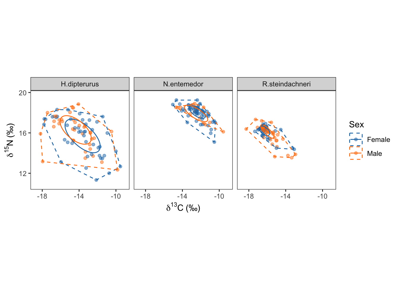

Eccentricities:

ecc <- data.frame()
for (sp in seq_along(species)) {
  for (j in seq_along(lbls)) {
    ecc <- rbind(ecc,
               data.frame(sp = species[sp],
                          j = lbls[j],
                          ecc = apply(sex_siber$ellips[[species[sp]]][[j]][,1:4], 1, mat_ecc),
                          theta = apply(sex_siber$ellips[[species[sp]]][[j]][,1:4], 1, mat_theta)))
    
  }
}

ec <- ecc %>% group_by(sp, j) %>% summarise(IQR.lower = hdi(ecc, credMass = 0.5)[1],
                                            IQR.upper = hdi(ecc, credMass = 0.5)[2],
                                            hdi.lower = hdi(ecc)[1],
                                            hdi.upper = hdi(ecc)[2],
                                            mean = mean(ecc))

`summarise()` has grouped output by 'sp'. You can override using the `.groups`
argument.

ec

ggplot(data = ecc, aes(x = j, y = ecc, group = j, color = factor(j))) +
  geom_violin(fill = NA, show.legend = F) +
  #geom_point(aes(x = sp, y = mean), data = ag, show.legend = F) +
  #geom_errorbar(aes(x = sp, ymin = IQ.lower, ymax = IQ.upper, group = sp), data = ag) +
  geom_boxplot(width = 0.1, show.legend = F) +
  theme_bw() +
  labs(title = "SEAB Eccentricity",
       x = element_blank(),
       y = element_blank()) +
  scale_color_manual(values = global_colors) +
  theme(aspect.ratio = 1,
                       panel.grid.major = element_blank(),
                       panel.grid.minor = element_blank(),
                       legend.position = c(0.15, 0.1),
                       legend.background = element_blank()) +
  facet_wrap(~sp)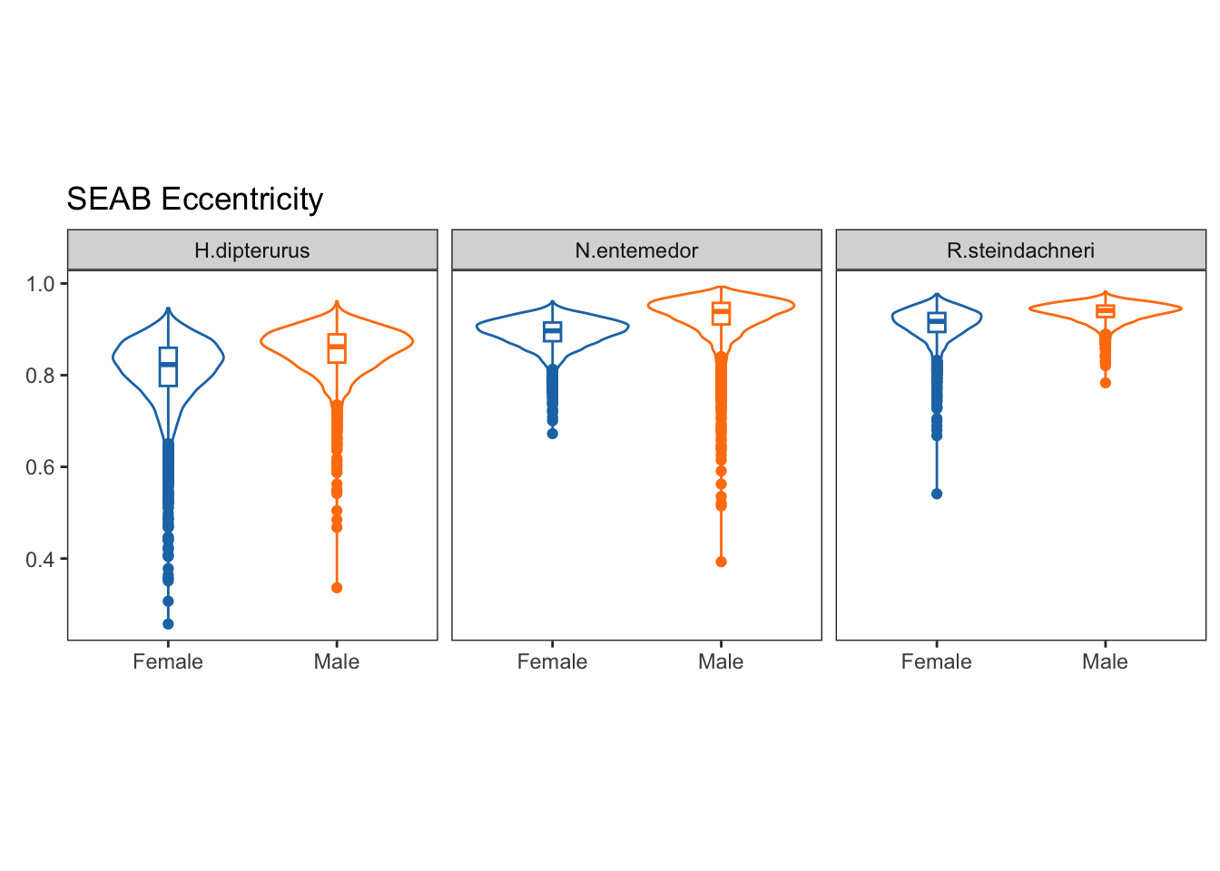

Theta:

th <- ecc %>% group_by(sp, j) %>% summarise(IQR.lower = hdi(theta, credMass = 0.5)[1],
                                            IQR.upper = hdi(theta, credMass = 0.5)[2],
                                            hdi.lower = hdi(theta)[1],
                                            hdi.upper = hdi(theta)[2],
                                            mean = mean(theta))

`summarise()` has grouped output by 'sp'. You can override using the `.groups`
argument.

th

ggplot(data = ecc, aes(x = j, y = theta, group = j, color = factor(j))) +
  geom_violin(fill = NA, show.legend = F) +
  #geom_point(aes(x = sp, y = mean), data = ag, show.legend = F) +
  #geom_errorbar(aes(x = sp, ymin = IQ.lower, ymax = IQ.upper, group = sp), data = ag) +
  geom_boxplot(width = 0.1, show.legend = F) +
  theme_bw() +
  labs(title = "SEAB theta",
       x = element_blank(),
       y = element_blank()) +
  scale_color_manual(values = global_colors) + 
  theme(aspect.ratio = 1,
                       panel.grid.major = element_blank(),
                       panel.grid.minor = element_blank(),
                       legend.position = c(0.15, 0.1),
                       legend.background = element_blank()) +
  facet_wrap(~sp)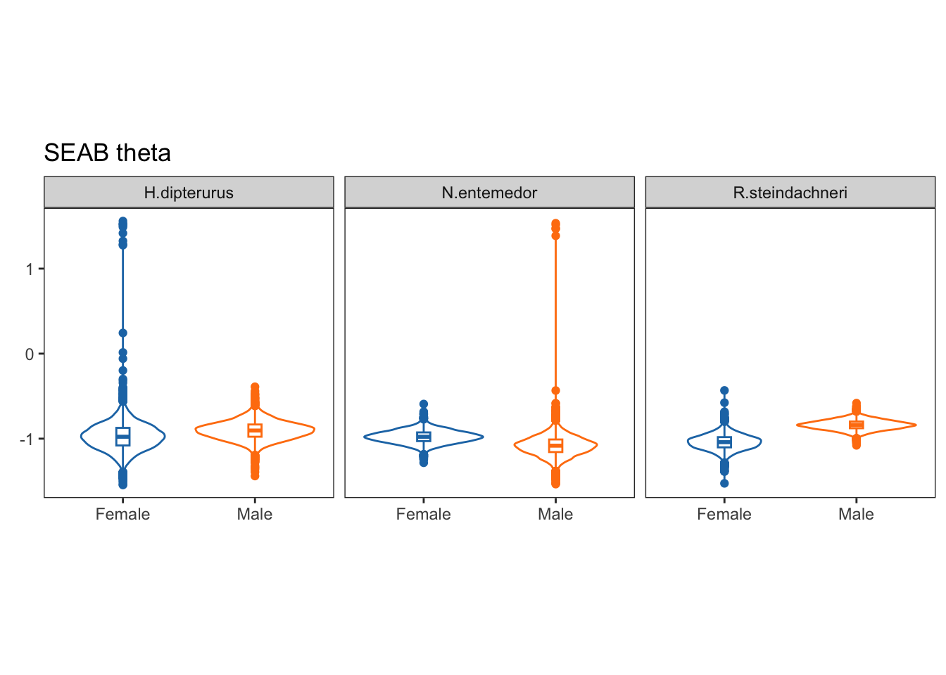

3.4.3 Maturity stages

lbls <- c("Adult", "Juvenile")
age_siber <- custom_siber(full_set, var_col = "Maturity", lbls, sp_col = "Species", n.burnin = 7000,
                          colors = global_colors, gp_label = "Age")

Compiling model graph
   Resolving undeclared variables
   Allocating nodes
Graph information:
   Observed stochastic nodes: 45
   Unobserved stochastic nodes: 3
   Total graph size: 60

Initializing model

Compiling model graph
   Resolving undeclared variables
   Allocating nodes
Graph information:
   Observed stochastic nodes: 36
   Unobserved stochastic nodes: 3
   Total graph size: 51

Initializing model

No id variables; using all as measure variables

Compiling model graph
   Resolving undeclared variables
   Allocating nodes
Graph information:
   Observed stochastic nodes: 55
   Unobserved stochastic nodes: 3
   Total graph size: 70

Initializing model

Compiling model graph
   Resolving undeclared variables
   Allocating nodes
Graph information:
   Observed stochastic nodes: 14
   Unobserved stochastic nodes: 3
   Total graph size: 29

Initializing model

No id variables; using all as measure variables

Compiling model graph
   Resolving undeclared variables
   Allocating nodes
Graph information:
   Observed stochastic nodes: 48
   Unobserved stochastic nodes: 3
   Total graph size: 63

Initializing model

Compiling model graph
   Resolving undeclared variables
   Allocating nodes
Graph information:
   Observed stochastic nodes: 26
   Unobserved stochastic nodes: 3
   Total graph size: 41

Initializing model

No id variables; using all as measure variables

[1] "All models have been run. Check your working directory for the results"

Plots of ellipses:

age_siber$ellips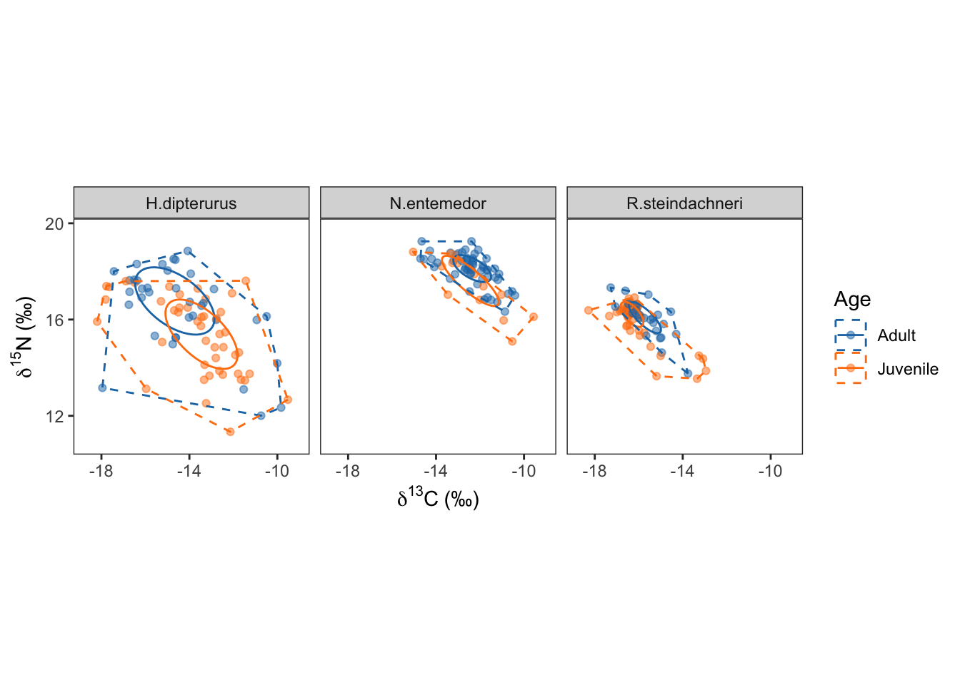

Eccenctricities:

ecc <- data.frame()
for (sp in seq_along(species)) {
  for (j in seq_along(lbls)) {
    ecc <- rbind(ecc,
               data.frame(sp = species[sp],
                          j = lbls[j],
                          ecc = apply(age_siber$ellips[[species[sp]]][[j]][,1:4], 1, mat_ecc),
                          theta = apply(age_siber$ellips[[species[sp]]][[j]][,1:4], 1, mat_theta)))
  }
}

ec <- ecc %>% group_by(sp, j) %>% summarise(IQR.lower = hdi(ecc, credMass = 0.5)[1],
                                            IQR.upper = hdi(ecc, credMass = 0.5)[2],
                                            hdi.lower = hdi(ecc)[1],
                                            hdi.upper = hdi(ecc)[2],
                                            mean = mean(ecc))

`summarise()` has grouped output by 'sp'. You can override using the `.groups`
argument.

ec

ggplot(data = ecc, aes(x = j, y = ecc, group = j, color = factor(j))) +
  geom_violin(fill = NA, show.legend = F) +
  #geom_point(aes(x = sp, y = mean), data = ag, show.legend = F) +
  #geom_errorbar(aes(x = sp, ymin = IQ.lower, ymax = IQ.upper, group = sp), data = ag) +
  geom_boxplot(width = 0.1, show.legend = F) +
  theme_bw() +
  labs(title = "SEAB Eccentricity",
       x = element_blank(),
       y = element_blank()) +
  scale_color_manual(values = global_colors) +
  theme(aspect.ratio = 1,
                       panel.grid.major = element_blank(),
                       panel.grid.minor = element_blank(),
                       legend.position = c(0.15, 0.1),
                       legend.background = element_blank()) +
  facet_wrap(~sp)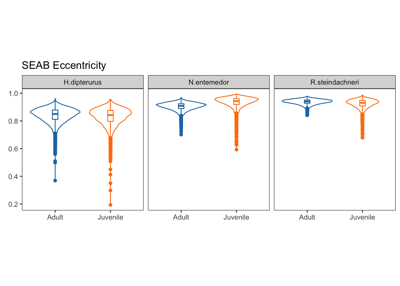

Theta:

th <- ecc %>% group_by(sp, j) %>% summarise(IQR.lower = hdi(theta, credMass = 0.5)[1],
                                            IQR.upper = hdi(theta, credMass = 0.5)[2],
                                            hdi.lower = hdi(theta)[1],
                                            hdi.upper = hdi(theta)[2],
                                            mean = mean(theta))

`summarise()` has grouped output by 'sp'. You can override using the `.groups`
argument.

th

ggplot(data = ecc, aes(x = j, y = theta, group = j, color = factor(j))) +
  geom_violin(fill = NA, show.legend = F) +
  #geom_point(aes(x = sp, y = mean), data = ag, show.legend = F) +
  #geom_errorbar(aes(x = sp, ymin = IQ.lower, ymax = IQ.upper, group = sp), data = ag) +
  geom_boxplot(width = 0.1, show.legend = F) +
  theme_bw() +
  labs(title = "SEAB theta",
       x = element_blank(),
       y = element_blank()) +
  scale_color_manual(values = global_colors) + 
  theme(aspect.ratio = 1,
                       panel.grid.major = element_blank(),
                       panel.grid.minor = element_blank(),
                       legend.position = c(0.15, 0.1),
                       legend.background = element_blank()) +
  facet_wrap(~sp)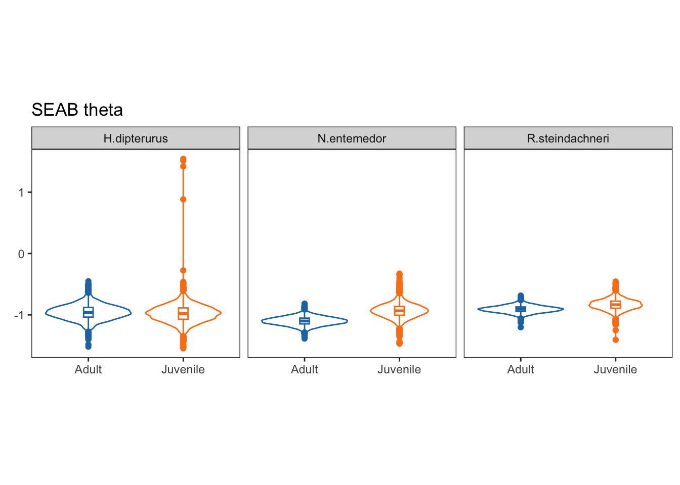

3.4.4 Season

lbls <- c("Warm", "Cold")
season_siber <- custom_siber(full_set, var_col = "Season", lbls, sp_col = "Species",
                             colors = global_colors, gp_label = "Season",
                             n.burnin = 750000, n.iter = 10000) 

Too few points to calculate an ellipse

Warning: Removed 1 row containing missing values (`geom_path()`).

Compiling model graph
   Resolving undeclared variables
   Allocating nodes
Graph information:
   Observed stochastic nodes: 63
   Unobserved stochastic nodes: 3
   Total graph size: 78

Initializing model

Compiling model graph
   Resolving undeclared variables
   Allocating nodes
Graph information:
   Observed stochastic nodes: 18
   Unobserved stochastic nodes: 3
   Total graph size: 33

Initializing model

No id variables; using all as measure variables

Compiling model graph
   Resolving undeclared variables
   Allocating nodes
Graph information:
   Observed stochastic nodes: 15
   Unobserved stochastic nodes: 3
   Total graph size: 30

Initializing model

Compiling model graph
   Resolving undeclared variables
   Allocating nodes
Graph information:
   Observed stochastic nodes: 54
   Unobserved stochastic nodes: 3
   Total graph size: 69

Initializing model

No id variables; using all as measure variables

Warning in createSiberObject(subdata[subdata[, sp_col] == species[i], 3:6]): At least one of your groups has less than 5 observations.
          The absolute minimum sample size for each group is 3 in order
          for the various ellipses and corresponding metrics to be 
          calculated. More reasonably though, a minimum of 5 data points
          are required to calculate the two means and the 2x2 covariance 
          matrix and not run out of degrees of freedom. Check the item 
          named 'sample.sizes' in the object returned by this function 
          in order to locate the offending group. Bear in mind that NAs in 
          the sample.size matrix simply indicate groups that are not 
          present in that community, and is an acceptable data structure 
          for these analyses.

Compiling model graph
   Resolving undeclared variables
   Allocating nodes
Graph information:
   Observed stochastic nodes: 71
   Unobserved stochastic nodes: 3
   Total graph size: 86

Initializing model

Compiling model graph
   Resolving undeclared variables
   Allocating nodes
Graph information:
   Observed stochastic nodes: 3
   Unobserved stochastic nodes: 3
   Total graph size: 18

Initializing model

No id variables; using all as measure variables

[1] "All models have been run. Check your working directory for the results"

Plots of ellipses:

season_siber$ellips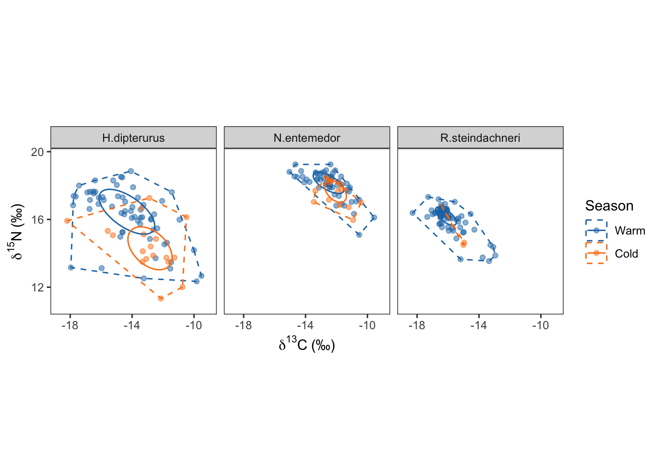

ecc <- data.frame()
for (sp in seq_along(species)) {
  for (j in seq_along(lbls)) {
    ecc <- rbind(ecc,
               data.frame(sp = species[sp],
                          j = lbls[j],
                          ecc = apply(season_siber$ellips[[species[sp]]][[j]][,1:4], 1, mat_ecc),
                          theta = apply(season_siber$ellips[[species[sp]]][[j]][,1:4], 1, mat_theta)))
  }
}

ec <- ecc %>% group_by(sp, j) %>% summarise(IQR.lower = hdi(ecc, credMass = 0.5)[1],
                                            IQR.upper = hdi(ecc, credMass = 0.5)[2],
                                            hdi.lower = hdi(ecc)[1],
                                            hdi.upper = hdi(ecc)[2],
                                            mean = mean(ecc))

`summarise()` has grouped output by 'sp'. You can override using the `.groups`
argument.

ec

ggplot(data = ecc, aes(x = j, y = ecc, group = j, color = factor(j))) +
  geom_violin(fill = NA, show.legend = F) +
  #geom_point(aes(x = sp, y = mean), data = ag, show.legend = F) +
  #geom_errorbar(aes(x = sp, ymin = IQ.lower, ymax = IQ.upper, group = sp), data = ag) +
  geom_boxplot(width = 0.1, show.legend = F) +
  theme_bw() +
  labs(title = "SEAB Eccentricity",
       x = element_blank(),
       y = element_blank()) +
  scale_color_manual(values = global_colors) +
  theme(aspect.ratio = 1,
                       panel.grid.major = element_blank(),
                       panel.grid.minor = element_blank(),
                       legend.position = c(0.15, 0.1),
                       legend.background = element_blank()) +
  facet_wrap(~sp)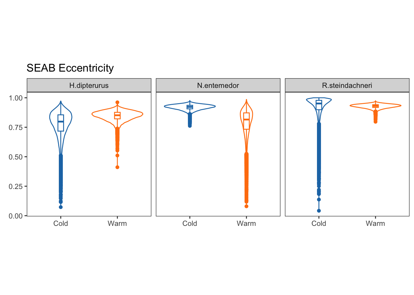

Theta:

th <- ecc %>% group_by(sp, j) %>% summarise(IQR.lower = hdi(theta, credMass = 0.5)[1],
                                            IQR.upper = hdi(theta, credMass = 0.5)[2],
                                            hdi.lower = hdi(theta)[1],
                                            hdi.upper = hdi(theta)[2],
                                            mean = mean(theta))

`summarise()` has grouped output by 'sp'. You can override using the `.groups`
argument.

th

ggplot(data = ecc, aes(x = j, y = theta, group = j, color = factor(j))) +
  geom_violin(fill = NA, show.legend = F) +
  #geom_point(aes(x = sp, y = mean), data = ag, show.legend = F) +
  #geom_errorbar(aes(x = sp, ymin = IQ.lower, ymax = IQ.upper, group = sp), data = ag) +
  geom_boxplot(width = 0.1, show.legend = F) +
  theme_bw() +
  labs(title = "SEAB theta",
       x = element_blank(),
       y = element_blank()) +
  scale_color_manual(values = global_colors) + 
  theme(aspect.ratio = 1,
                       panel.grid.major = element_blank(),
                       panel.grid.minor = element_blank(),
                       legend.position = c(0.15, 0.1),
                       legend.background = element_blank()) +
  facet_wrap(~sp)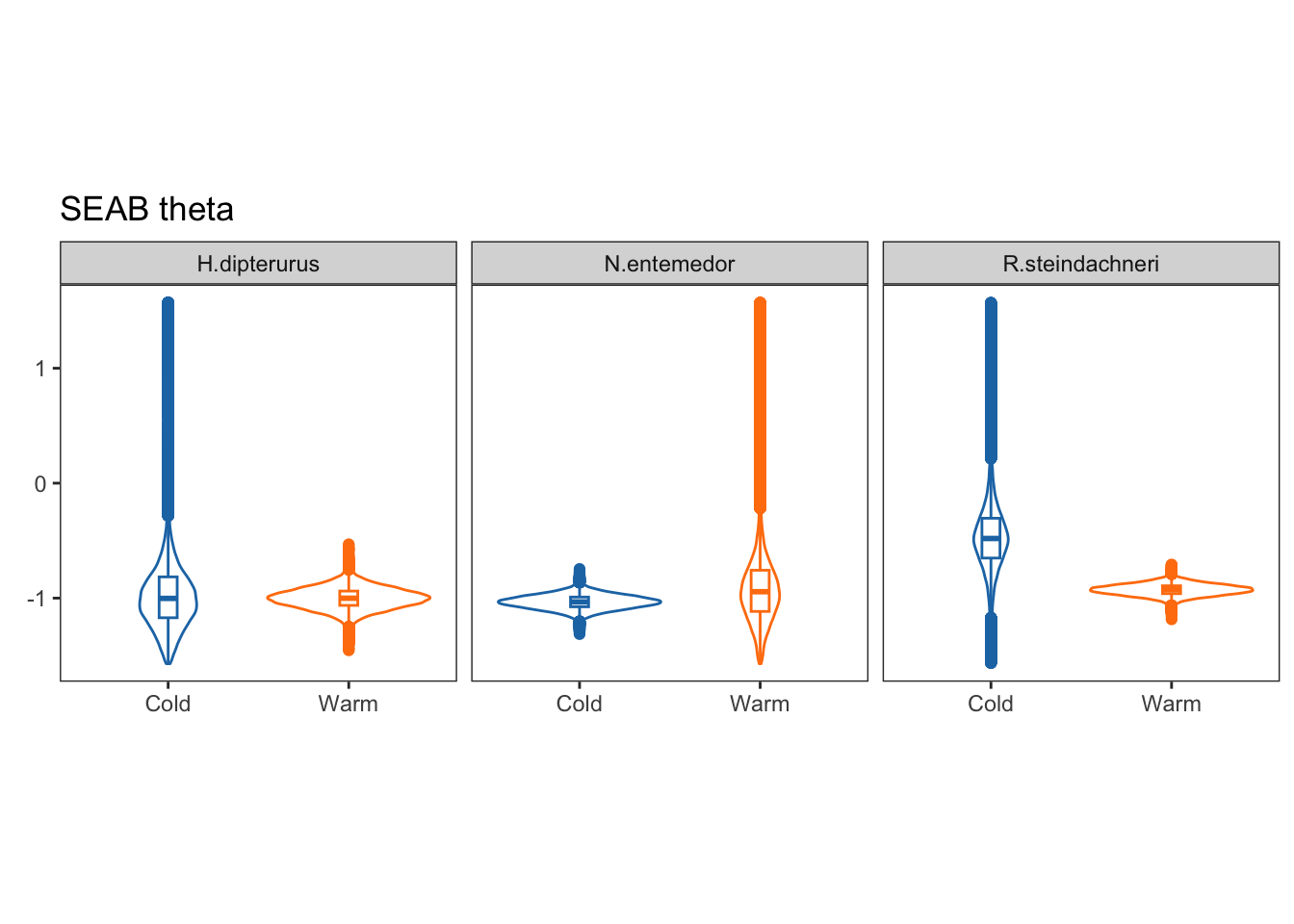

3.4.5 Final forestplot:

forest_data <- rbind(age_siber[[6]], season_siber[[6]], sex_siber[[6]])

forest <- ggplot(data = forest_data) +
               geom_vline(xintercept = 0, linetype = "dashed", color = "#C9C8C8", size = 0.5) +
               geom_linerange(aes(y = comp, xmin = IQr.lower, xmax = IQr.upper),
                              color = global_colors[1], size = 1) +
               geom_linerange(aes(y = comp, xmin = hdi.lower, xmax = hdi.upper),
                              color = global_colors[1]) +
               geom_point(aes(x = mean, y = comp),
                          color = global_colors[1], fill = "white", size = 1.5, shape = 21) +
               theme_bw() +
               theme(aspect.ratio = 1,
                     panel.grid.major = element_blank(),
                     panel.grid.minor = element_blank(),
                     legend.position = c(0.2, 0.15),
                     legend.background = element_blank()) +
               scale_x_continuous(breaks = scales::pretty_breaks(n = 3)) +
               labs(title = element_blank(),
                    x = element_blank(),
                    y = element_blank()) + facet_wrap(~sp)

# cairo_pdf("output/SIBER/forest_cats.pdf", family = "Times", width = 4, height = 2)
forest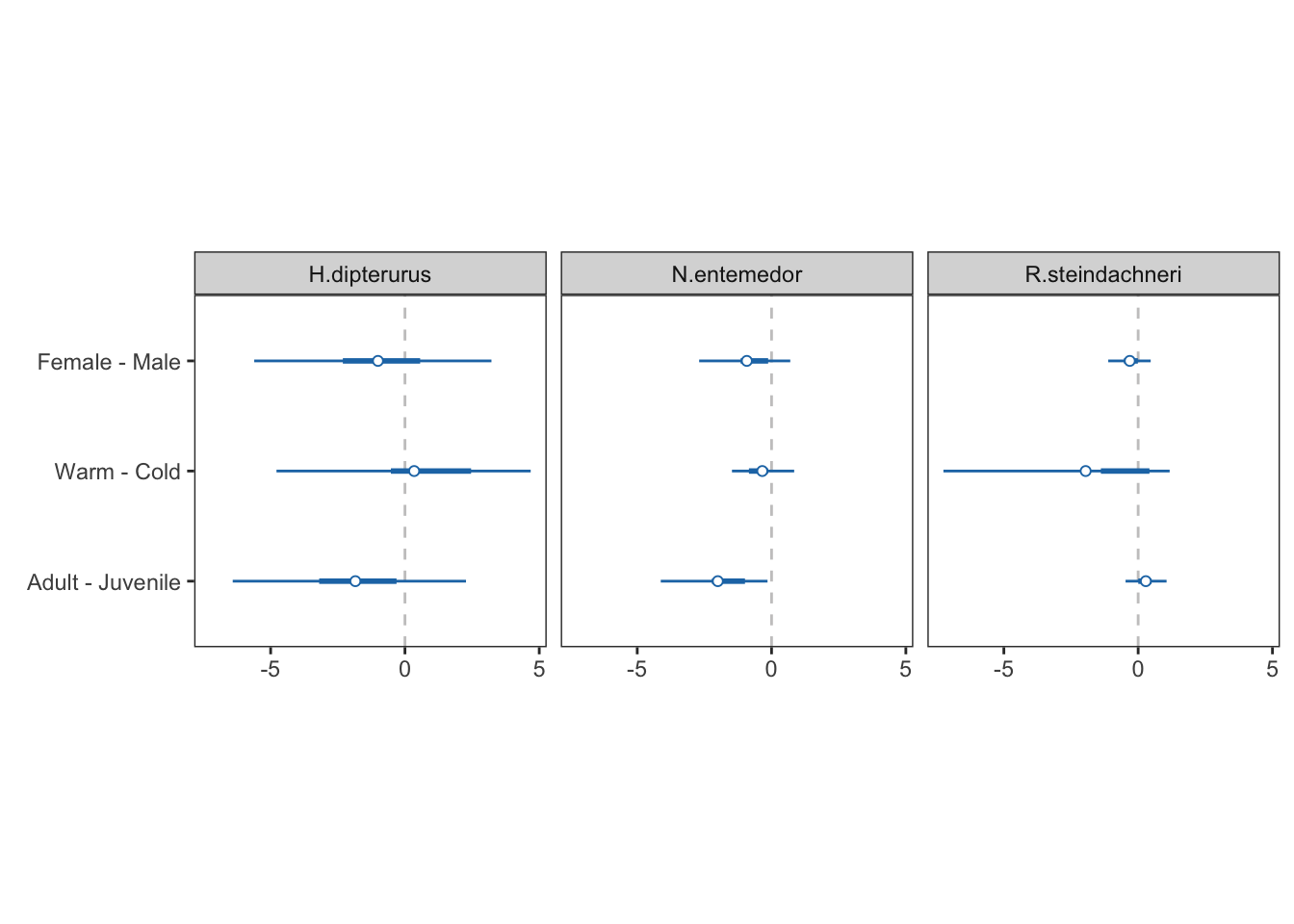

# dev.off()

Tabular results:

Seasons:

season_siber$diff_glob[,c("comp", "sp", "mean")]

season_siber$p_sup

Sexes:

sex_siber$diff_glob[,c("comp", "sp", "mean")]

sex_siber$p_sup

Maturity stages:

age_siber$diff_glob[,c("comp", "sp", "mean")]

age_siber$p_sup